
1.Introduction
Two-dimensional Runoff Inundation Toolkit for Operational Needs (TRITON)
This document serves as a User’s Guide for Two-dimensional Runoff Inundation Toolkit for Operational Needs (TRITON; Morales-Hernández et al., 2021), which is a two-dimensional (2D) hydrodynamic model that simulates flood wave propagation and surface inundation based on the full shallow water equations. The purpose of this document is to provide new users with key information about the model and help them navigate through various topics including how to download, install and run the code. This guide also provides information about input and output files, model features and provides step by step instruction on simulating the pre-designed test cases or configure users’ own simulation. Users are recommended to refer to technical reference manual for more advanced and detailed information.
Morales-Hernández, M., Sharif, M.B., Kalyanapu, A., Ghafoor, S.K., Dullo, T.T., Gangrade, S., Kao, S.C., Norman, M.R. and Evans, K.J., 2021. TRITON: A Multi-GPU Open Source 2D Hydrodynamic Flood Model. Environmental Modelling & Software, p.105034, https://doi.org/10.1016/j.envsoft.2021.105034.
2.Overview
The Two-dimensional Runoff Inundation Toolkit for Operational Needs (TRITON; Morales-Hernández et al., 2021) is a 2D open source flood simulation tool designed for modern high performance computing (HPC). The core of the tool is a computationally efficient, physics-based hydraulic model that operates on a regular/structured grid and solves the full 2D shallow water equations. The key features of TRITON are:
- It can operate on multiple computer platforms and utilize modern HPC environments.
- The users can take advantage of:
- Implementation with a single central processing unit (CPU) or multiple CPUs (using OpenMP+MPI)
- Implementation with a single graphics processing unit (GPU) or multiple GPUs (using CUDA+MPI)
- Highest TRITON computational efficiency can be achieved by using GPU implementation.
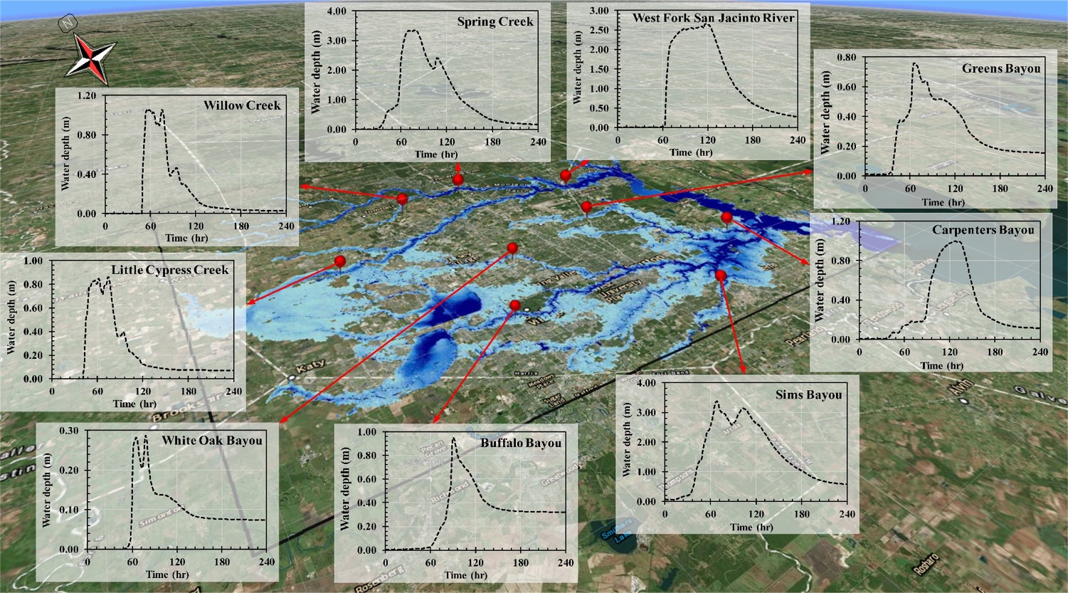
- TRITON utilizes topographical data (e.g., digital elevation model [DEM], light detection and ranging [LIDAR]), as its base input, in a uniform (Cartesian) grid structure. The model can be driven by streamflow hydrographs at specified locations or gridded runoff hydrographs, or both which serves as the model’s hydrological forcing. The primary TRITON output includes water depth and 2D unit discharge maps at user defined time intervals. Other variables such as unit discharge values can be outputted. TRITON can also output timeseries of simulated results as user-defined point locations. An example is shown below:
- TRITON is developed on Linux/Unix platform. The input/output files can be either in ascii or binary formats. A set of tools and instruction are provided for format conversion.
- The model utilizes International System of Units (SI). Users who are more familiar with United States (US) customary units need to perform proper unit conversion themselves.
A 2D open source flood simulation tool designed for modern high performance computing (HPC). The core of the tool is a computationally efficient, physics-based hydraulic model that operates on a regular/structured grid and solves the full 2D shallow water equations. The key features of TRITON are:
Morales-Hernández, M., Sharif, M.B., Kalyanapu, A., Ghafoor, S.K., Dullo, T.T., Gangrade, S., Kao, S.C., Norman, M.R. and Evans, K.J., 2021. TRITON: A Multi-GPU Open Source 2D Hydrodynamic Flood Model. Environmental Modelling & Software, p.105034, https://doi.org/10.1016/j.envsoft.2021.105034.
3.License and Availability
- Name of the software: TRITON (Two-dimensional Runoff Inundation Toolkit for Operational Needs)
- Contact address: Oak Ridge National Laboratory, 1 Bethel Valley Road, TN 37830, USA / Tennessee Technological University, 1 William L Jones Dr, Cookeville, TN 38505, USA
- Email: Mario Morales-Hernández ([email protected]), Alfred Kalyanapu ([email protected])
- Language: CUDA, C++
- Hardware: Desktop/Laptop or clusters of CPUs/GPUs
- Software: NVIDIA CUDA Toolkit, NETCDF (optional)
- Availability: https://code.ornl.gov/hydro/triton
- Year first available: 2020
- Copyright (c) 2019, UT-Battelle, LLC and Tennessee Technological University. All rights reserved.
Redistribution and use in source and binary forms, with or without modification, are permitted provided that the following conditions are met: 1. Redistributions of source code must retain the above copyright notice, this list of conditions and the following disclaimer. 2. Redistributions in binary form must reproduce the above copyright notice, this list of conditions and the following disclaimer in the documentation and/or other materials provided with the distribution. 3. Neither the name of the copyright holder nor the names of its contributors may be used to endorse or promote products derived from this software without specific prior written permission.
THIS SOFTWARE IS PROVIDED BY THE COPYRIGHT HOLDERS AND CONTRIBUTORS “AS IS” AND ANY EXPRESS OR IMPLIED WARRANTIES, INCLUDING, BUT NOT LIMITED TO, THE IMPLIED WARRANTIES OF MERCHANTABILITY AND FITNESS FOR A PARTICULAR PURPOSE ARE DISCLAIMED. IN NO EVENT SHALL THE COPYRIGHT HOLDER OR CONTRIBUTORS BE LIABLE FOR ANY DIRECT, INDIRECT, INCIDENTAL, SPECIAL, EXEMPLARY, OR CONSEQUENTIAL DAMAGES (INCLUDING, BUT NOT LIMITED TO, PROCUREMENT OF SUBSTITUTE GOODS OR SERVICES; LOSS OF USE, DATA, OR PROFITS; OR BUSINESS INTERRUPTION) HOWEVER CAUSED AND ON ANY THEORY OF LIABILITY, WHETHER IN CONTRACT, STRICT LIABILITY, OR TORT (INCLUDING NEGLIGENCE OR OTHERWISE) ARISING IN ANY WAY OUT OF THE USE OF THIS SOFTWARE, EVEN IF ADVISED OF THE POSSIBILITY OF SUCH DAMAGE.
4.Obtaining the Source Code
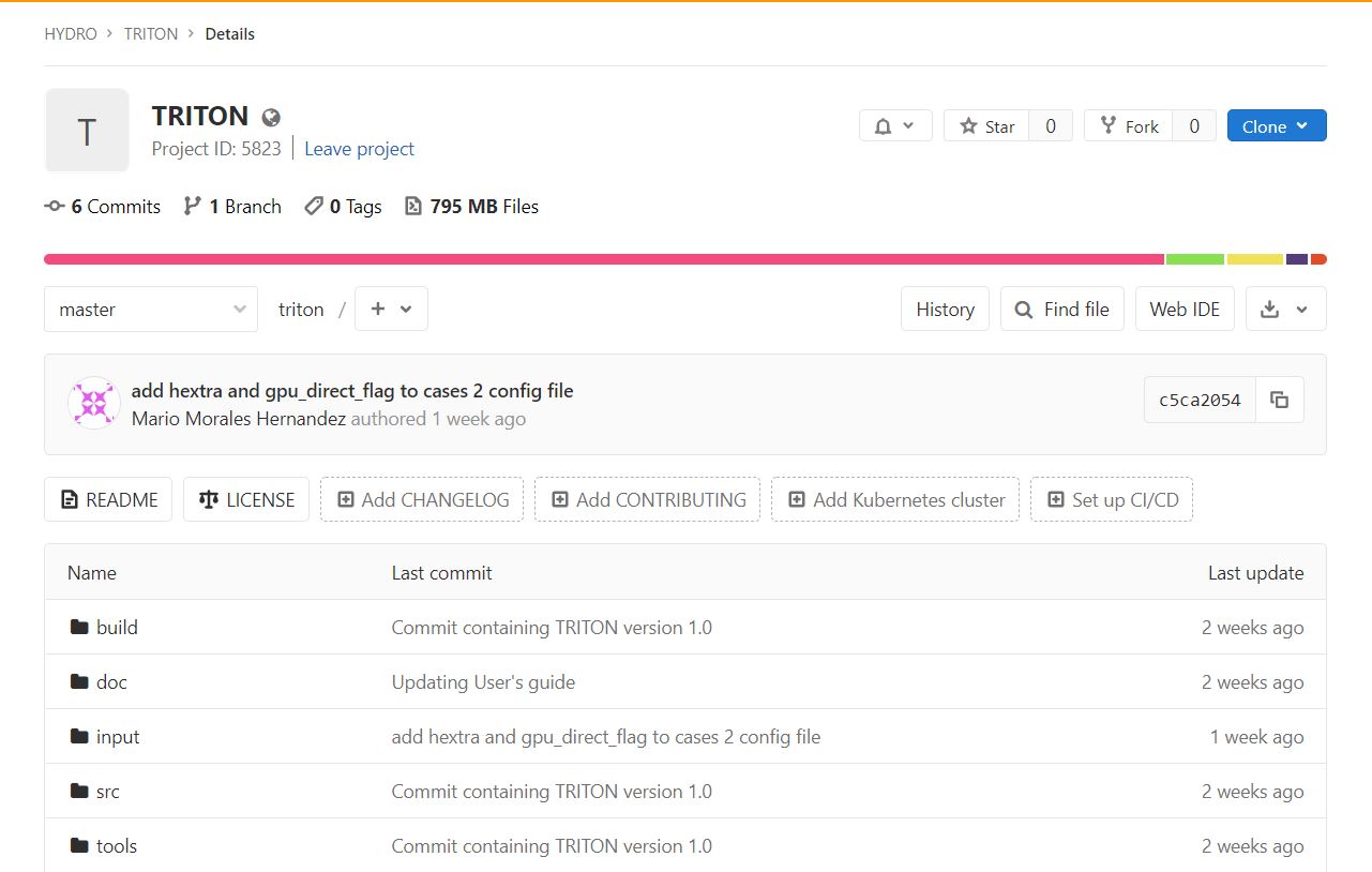
The source code is available via several mechanisms. Users can obtain the code and pre-designed test cases using of the one of the following approaches. a. The latest version of code is maintained on the git repository. The packed archive file of the code and test cases is available to download from https://code.ornl.gov/hydro/triton . A user can download a tar.gz file from the website (as shown in the figure below) or in any other format as appropriate.
Assuming the downloaded file is named triton-master.tar.gz, use the following commands in terminal.
Use the following commands to unpack the file
tar -xzvf triton-master.tar.gz
cd triton-master
Hereafter, within this document, this directory will be referred as $TRITON.
Alternatively, users can directly clone the repository using the following commands
mkdir $TRITON
cd $TRITON
git clone https://code.ornl.gov/hydro/triton.git
cd triton
Hereafter, within this document, this directory will be referred as $TRITON. To explore the directory structure, refer to Section 5.
5.Building the Executable
OLCF supercomputer – Summit
For GPU implementation
To create required environment, use the following commands
cd $TRITON
module load cuda
make clean && make summit_gpu
If successful, the executable triton will be located in the $TRITON/build folder.
For CPU (OpenMP) implementation
To create required environment, use the following commands
cd $TRITON
module load gcc
make clean && make summit_omp
If successful, the executable triton will be located in the $TRITON/build folder.
Non-OLCF machine
If you are using a Linux based machine, changes are required to the makefile.hpc to compiler flags in the file. The GPU based implementation requires nvcc compiler, while openMP requires gcc compiler.
The makefile.hpc contains following information:
ifdef ACTIVE_GPU
	CC := nvcc
	INC_DIRS :=
	FLAGS := --compiler-bindir `which mpic++` -arch=sm_35 -x cu
	LIBRARIES :=
	DFLAGS := -DACTIVE_GPU=1
else
	CC := mpic++
	INC_DIRS :=
	FLAGS := -Wall -fopenmp
	LIBRARIES :=
	DFLAGS := -DACTIVE_OMP=1
endif

triton: src/main.cpp
	if [ ! -d "build" ]; then mkdir build; fi
	@echo 'Compiling file: $<'
	$(CC) $(INC_DIRS:%=-I%) $(FLAGS) $(DFLAGS) -O3 $(LIBRARIES) -o "build/$@" "$<" --std=c++11
	@echo 'Building finished: $@'
For GPU implementation
Use the following commands
cd $TRITON
make clean && make hpc_gpu
If successful, the executable triton will be located in the $TRITON/build folder.
For CPU (OpenMP) implementation
Use the following commands
cd $TRITON
make clean && make hpc_omp
If successful, the executable triton will be located in the $TRITON/build folder.
6.Running the Executable
The basic command to run the simulation is:
cd $TRITON
./build/triton $CFG_NAME
where,
$CFG_NAME = Config file name
OLCF supercomputer – Summit
cd $TRITON
jsrun -n $N -r $R -a $A -g $G -c $C --smpiargs="-gpu" \ ./build/triton $CFG_NAME
where,
$N = Number of total resources
$R = Number of resources per node
$A = Number of MPI process per resource
$G = Number of GPU per resource
$C = Number of CPU per resource
$CFG_NAME = Config file name
Non-OLCF machine
cd $TRITON
mpirun -n ./build/triton $CFG_NAME
7.Main Directory Structure
The main directory structure and contents are described in this section.
$TRITON         : top level base directory
|--build        : contains the executable
|--doc  : documentation (User guide, Reference Manual)
|--input                : input data, parameters and forcing directory
   |--cfg               : configuration file directory
   |--dem               : elevation data directory
   |--extbc     : external boundary conditions directory
   |--initc     : initial depths and unit discharge conditions
          |--inith
          |--initqx
          |--initqy
   |--mann              : manning’s roughness coefficient parameters
   |--stageloc  : user defined locations at which timeseries water elevation output is desired
   |--runoff    : runoff map and timeseries forcing
   |--strmflow  : streamflow hydrograph and locations
|--output               : output data is generated here
|--src          : contains the source code
|--tools        : contains miscellaneous utilities for pre and post processing data for TRITON
8.TRITON Configuration
The TRITON simulation can be configured and controlled by the configuration file which is located in the $TRITON/input/cfg subdirectory. The configuration file is a text file used to control various simulation options such as duration, parameters, paths to input and output, etc.
As a new user we recommend you explore one of the pre-existing configuration files to get acquainted. To configure your own test case, use one of these files as a template and make appropriate changes as necessary. A quick walk-through of main contents of the configuration file is provided.
Topography
dem_filename: Path where DEM is located.
Example Usage:
dem_filename="input/dem/asc/dem_file.dem"
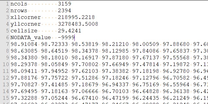
TRITON accepts topographical data in Esri ASCII raster format. This file contains first six rows as header information, followed by a space delimited matrix of nrows x ncols (an example snapshot of the file is shown below). This serves as the base computational domain for the hydraulic simulations where the number of rows and columns defines the size of the computational domain.
Refer to $TRITON/input/dem to explore provided DEM examples.
Note: When designing a simulation, users must exercise caution to avoid having negative NODATA values (e.g. NODATA_value = -9999) in the topographical data, as they will act as large depressions during the hydraulic simulations.
Surface Roughness (Manning’s n Coefficient)
n_infile: location of manning’s roughness file
Example Usage:
n_infile="input/mann/asc/roughness_file.mann"
TRITON accepts spatially varying Manning’s n coefficient to account for surface roughness. The roughness should be defined explicitly for each grid cell of the computational domain. Therefore, this file follows the same template as of the DEM file (explained above) excluding the header (i.e., ESRI ASCII raster format, but without the header).
const_mann: =user defined constant Manning’s n value
Example Usage:
const_mann=0.035
Alternatively, user can also decide to provide a constant Manning’s n value to the entire computational domain.
Hydrologic Forcing
TRITON can be driven by either providing streamflow hydrographs at specified locations or gridded runoff hydrograph, or both which serve as the model’s hydrological forcings.
Streamflow Hydrograph
hydrograph_filename: file location of streamflow hydrograph
Example usage
hydrograph_filename="input/strmflow/streamflow.hyg"
This file contains the streamflow hydrograph information. This data is in form of a table including the time (in hours), as first column. This is followed by columns of inflow sources (equal to number of inflow locations), containing the discharge for each source. The units must be in cubic meters per second (m3/s).
num_sources: number of inflow points/locations
Example usage
num_sources=2
src_loc_file: file with cartesian coordinates of inflow locations.
Example usage
src_loc_file="input/strmflow/location.txt"
This file contains cartesian coordinates of all the inflow locations, in the order they appear in the hydrograph_filename.
Runoff Hydrograph
Users can also decide to provide runoff as an alternative or along with streamflow as an input hydrologic forcing to the TRITON.
• runoff_filename: file location with runoff hydrograph
Example usage
runoff_filename="input/runoff/runoff.hyg"
Note: This file contains the runoff hydrograph information. This file contains data in form of a table including the time (in hours), as first column. This is followed by columns of runoff sources (equal to number of inflow locations), containing the discharge evolution for each source. The units should be in mm per hour (mm/hour).
num_runoffs: number of distinct runoff areas
Example usage
num_runoffs=156
runoff_map: matrix raster map of distinct areas
Example usage
runoff_map="input/runoff/runoff.rmap"
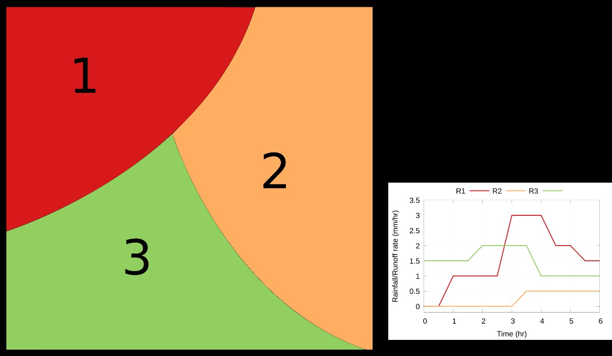
This file follows the same template as of the DEM file (explained above) excluding the header (i.e., ESRI ASCII raster format, but without the header). The file is a spatial map of distinct runoff areas defined by a non-negative integer number for each grid cell in the computational domain.
A sketch of the rainfall/runoff input files is depicted below, for a more detailed explanation please refer to Morales-Hernández et al., XX or explore the input files of test case #3.
External Boundary
num_extbc: number of external boundary conditions
Example usage
num_extbc=0
If num_extbc = 0, by default, boundaries of the computational domain (north, east, south and west) are assumed closed (i.e., water flow is prevented to cross out the domain) If num_extbc = 1 or greater, the boundary conditions are controlled by extbc_file
extbc_file: file to control the external boundary conditions
Example usage
extbc_file="input/extbc/boundary.extbc"
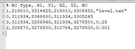
In this file, the first column represents boundary condition type. Currently, boundary can acquire one of the following values 0, 1, 2 or 3. A brief description of each type is given below
0: free flow (supercritical). No additional files are required.
1: level versus time. An additional file containing a table with the time and the water level is mandatory.
2: normal slope. The desired slope value is required in the last column.
3: Froude number. The Froude number to be imposed across the external boundary is required in the last column.
The second through fifth column represents X and Y coordinates of the two points between which a boundary is to be implemented.
An example of extbc_file is given below:
Simulation Control
sim_start_time: start time of simulation in seconds
Example usage
sim_start_time=0
sim_duration: duration of simulation in seconds
Example usage
sim_start_time=43200
checkpoint_id= checkpoint id.
The checkpoint id can be used to restart a simulation. The checkpoint id is a counter written in the file $TRITON/cid once the simulation starts. The counter increases after every print interval. This is especially helpful if the simulation was not complete for any reason, and user would like to start from a particular point to avoid rerunning the entire simulation. The default value is zero, assuming a clean start.
To restart the simulation from a checkpoint, user must output all huv maps in the print_option as described in the Output section
Example usage
checkpoint_id = 24
time_increment_fixed= switch to control the time step.
Example usage
time_increment_fixed=0 for variable dt
time_increment_fixed=1 for constant dt
If time_increment_fixed=1
Then use time_step variable to control the timestep size. The units are in seconds.
Example UsageExample usage
time_step=0.01
If a user is interested to start the simulation using initial condition, the following maps can be provided.
h_infile = initial water depth file qx_infile = initial x direction unit discharge file qy_infile = intial y direction unit discharge file
Example usage
h_infile="input/inith/asc/case5.inith"
qx_infile="input/initqx/asc/case5.initqx"
qy_infile="input/initqy/asc/case5.initqy"
Output Control
print_option= switch to govern the type of output
Example usage
print_option=h  % to output water elevation maps only
print_option=huv % to output water
A map for the water depth (h) and unit discharges (uv) is written in the form of an ESRI ASCII raster file (without header) as controlled by print_interval. This information can be written either in ASCII or in binary –the latter is recommended for large scale domains.
print_interval= number of seconds after which the outputs will be saved.
Example usage
print_interval = 1800 % outputs will be saved every 1800 seconds in the simulation, throughout the duration of simulation.
time_series_flag= switch to activate or deactivate the output of water stage hydrographs at user defined locations.
Example usage
time_series_flag=0 % to deactivate this option
time_series_flag=1 % to activate
If time_series_flag=1 provide information about observation_loc_file
observation_loc_file: file containing coordinates of the user-defined locations where output is desired.
Input Output File Settings
The model deals with two different type of file types – ASCII or Binary. The type of input or output files can be controlled in this section. A conversion tools between ascii and binary file types is detailed in Section 8. The user can decide suitable file type using the following controls.
Example usage
input_format=ASC   # Possible options BIN or ASC
output_format=ASC
The user can decide suitable file type using the following controls. .. code-block:: bash
outfile_pattern=”%s/%s/%s_%02d_%02d” # controls file naming convention output_option=PAR # Possible options PAR or SEQ
A switch in the configuration file allows the user to choose the mode in which the data is written. SEQ sequentially, i.e., gathering all the subdomains in a single file during the computation PAR in parallel
Other Miscellaneous parameters
courant= Courant-Friedrichs-Lewy (CFL) number
Example usage
courant=0.5
According to the stability condition, this value should not exceed 0.5
hextra= water depth tolerance value below which velocities are set to zero
Example usage
hextra=0.001
gpu_direct_flag= this parameter should be set to 0 unless your system has multiple GPUs with CUDA-Aware MPI implemented on it. In that case, the value can be set to 1 to get maximum performance
Example usage
gpu_direct_flag=0
9.Test Cases Overview
A set of test cases are provided with the TRITON release, detailed in Morales-Hernández et al., in preparation. These test cases provide examples of real-world like examples and are aimed to highlight different capabilities of the model and its performance. The configuration file for each case is available at :
$TRITON/input/case01.cfg  : Case 1  – TaumSauk Dam Failure
$TRITON/input/case02a.cfg : Case 2a – Paraboloid (0.04m)
$TRITON/input/case02b.cfg : Case 2b – Paraboloid (0.02m)
$TRITON/input/case02c.cfg : Case 2c – Paraboloid (0.01m)
$TRITON/input/case02d.cfg : Case 2d – Paraboloid (0.005m)
$TRITON/input/case03.cfg  : Case 3  – Runoff + Streamflow
$TRITON/input/case04.cfg  : Case 4  – Hurricane Harvey (30m)
$TRITON/input/case05.cfg  : Case 5  - Hurricane Harvey (10m)
Note : Please note that Cases 1 and 2a are ideal for quick testing on single CPU based machines. Case 3, 4 and 5 are medium to large scale cases only suitable for HPC machines or GPU based machines.
Case 1 : This test case is an example of dam failure simulation. For more details refer to Kalyanapu et al., 2011.
Case 2 : Test case 2a through 2d is a test case with a frictionless paraboloid topography using four different grid resolutions of 0.04, 0.02, 0.01 and 0.005m. This test case is detailed in Section 5.1 of Morales-Hernández et al. (in preparation).
Case 3 : Test case designed to simulate a 5-day flood event, using both streamflow and runoff as the hydrologic drivers. This test case is detailed in Section 5.2 of Morales-Hernández et al. (in preparation).
Case 4 : Test case designed to simulate a 10-day flood event during Hurricane Harvey over Harris County, TX, with a 30 m grid resolution. This case is a variant of Case 5 which uses 10 m grid resolution.
Case 5 : Test case designed to simulate a 10-day flood event during Hurricane Harvey over Harris County, TX, with a 10 m grid resolution. This test case is detailed in Section 5.2 of Morales-Hernández et al. (in preparation).
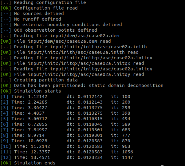
On successful building of the executable, any of the given cases can be used. On successful simulation execution, users can expect to see similar messages on their screen.
10.Other Tools
A set of utility tools are provided to ease the pre and postprocessing of the input/output files. These tools are located in $TRITON/tools/
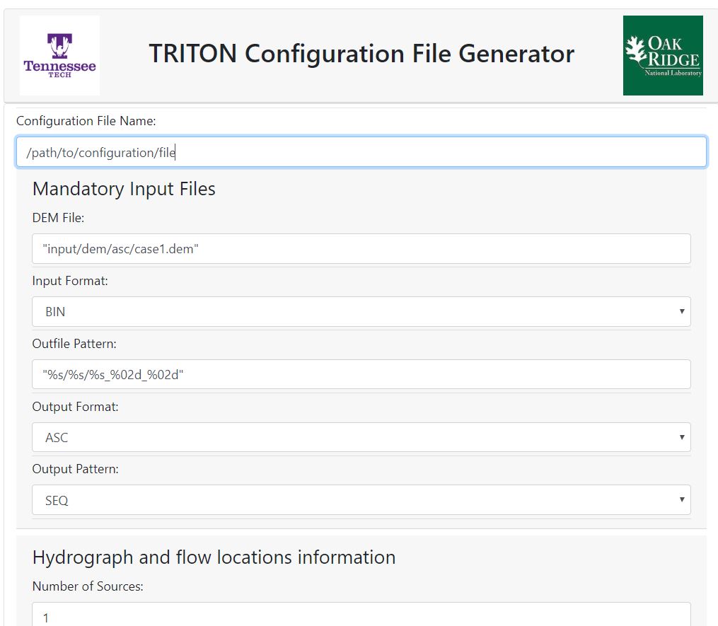
Configuration File Generator
This tool provides a graphical user interface to create the configuration file for TRTION. It is currently supported only for the Windows machines. To use this tool, run the executable “main” from the following location $TRITON/tools/ConfigGenerator/Windows EXE/. When launched successfully, this executable will open a localhost web browser and show a user interface. Provide necessary information (as shown below, as an example), and click Generate Config button to download the newly created configuration file. Alternatively, users can start with one of the pre-existing configuration files from the test cases and modify per their needs.\
Ascii to Binary Conversion
This tool converts ascii files (without header) to binary format.
cd $TRITON/tools/ascii2bin
module load gcc
make clean && make
./ascii2bin $INPUT_DIR $OUTPUT_DIR $TYPE
Where, $INPUT_DIR = Input file/folder directory of Ascii files $OUTPUT_DIR = Output file/folder directory of Binary files $TYPE = 1 for single file conversion , 2 to convert all the files in the input folder If the ascii files contains header, use the $TRITON/tools/ascii2bin_dem folder.
Binary to Ascii Conversion
This tool converts binary files to ascii format.
cd $TRITON/tools/bin2ascii
module load gcc
make clean && make
./ascii2bin $INPUT_DIR $OUTPUT_DIR $TYPE
Where,
$INPUT_DIR = Input file/folder directory of Ascii files $OUTPUT_DIR = Output file/folder directory of Binary files $TYPE = 1 for single file conversion , 2 to convert all the files in the input folder
Discharge to Velocity Conversion
This tool enables conversion of discharge files to velocity.
cd $TRITON/tools/discharge2velocity
module load gcc
make clean && make
./discharge2velocity $INPUT_DIR $FILE_TYPE $TYPE
Where, $INPUT_DIR = Input file/folder directory of discharge $OUTPUT_DIR = Output file/folder directory of velocity $FILE_TYPE = 1 for Ascii, 2 for Binary $TYPE = 1 for file, 2 for folder
Join Utility
If users enable output_option=PAR , the join utility can be used as a postprocessing tool, to create a merged ascii outputs i.e. a single output file for every print interval. The input files should be located in the $TRITON/output/asc folder.
ASCII/Binary to NetCDF Conversion
This tool located in $TRITON/tools/NetCDFconvertor, allows users to convert the files from ASCII/Binary format to NetCDF format.
Windows:
Execute the “main.exe” file.
Linux:
For Linux based implementation, following dependencies are required. Python3, Python-netCDF4, Python-eel, Python-Tkinter
cd $TRITON/tools/NetCDFconvertor/Linux EXE/
./main
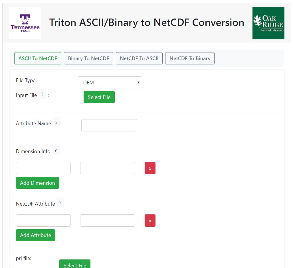
To convert a file, first select one of the “ASCII to NETCDF” or “Binary to NETCDF” button on the top (as shown in the example below). Next, selected the input file type using the dropdown button. The option ‘DEM’ refers to files with header information. If the header is missing from the input file, use the ‘other’ option. Select the input file using the “Select File” Button. In case of DEM file, the dimension and attributes will be obtained from the header automatically.User can provide the “attribute name”, which will be the variable in the NetCDF file and projection file information. Finally clicking “Generate” button will allow user to navigate to deseired directory and save the NetCDF file.
11.References and Related Publications
Morales-Hernández, M., Sharif, M.B., Kalyanapu, A., Ghafoor, S.K., Dullo, T.T., Gangrade, S., Kao, S.C., Norman, M.R. and Evans, K.J., 2021. TRITON: A Multi-GPU Open Source 2D Hydrodynamic Flood Model. Environmental Modelling & Software, p.105034, https://doi.org/10.1016/j.envsoft.2021.105034.
Kalyanapu, A. J., Shankar, S., Pardyjak, E. R., Judi, D. R., & Burian, S. J. (2011). Assessment of GPU computational enhancement to a 2D flood model. Environmental Modelling & Software, 26(8), 1009-1016.
Dullo, T.T., Gangrade, S., Morales‐Hernández, M., Sharif, M.B., Kao, S.C., Kalyanapu, A.J., Ghafoor, S. and Evans, K.J., 2021. Simulation of Hurricane Harvey flood event through coupled hydrologic‐hydraulic models: Challenges and next steps. Journal of Flood Risk Management, p.e12716, https://doi.org/10.1111/jfr3.12716.
Sharif, M.B., Ghafoor, S.K., Hines, T.M., Morales-Hernändez, M., Evans, K.J., Kao, S.C., Kalyanapu, A.J., Dullo, T.T. and Gangrade, S., 2020, June. Performance Evaluation of a Two-Dimensional Flood Model on Heterogeneous High-Performance Computing Architectures. In Proceedings of the Platform for Advanced Scientific Computing Conference (pp. 1-9), doi:10.1145/3394277.3401852.
12.Frequently Asked Questions
1. Can TRITON be used for Windows based machines ?
Currently, TRITON is developed for Linux/Unix platform. The future releases may include a Windows based version.
2. What is the unit system used by TRITON ?
The model utilizes International System of Units (SI). Users who are more familiar with United States (US) customary units need to perform proper unit conversion themselves.